Generating time series for Ordinary Differential Equations

Ordinary Differential Equations (ODEs) can be used to define systems in fields as varied as biology to engineering to mathematics. These equations express a relationship between an unknown function and its derivative. One example, the Rossler attractor:

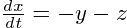
A short time series from the Rosseler Attractor

We can produce a time series from these equations by solving the equations using the iterative 4-th order Runge-Kutta method and plugging each of the solutions back into the equations. Along with the following script which allows you to implement the Runge-Kutta method on ODEs, I have included code to numerically estimate the largest Lyapunov exponent. The largest Lyapunov exponent is used to indicate chaos, or sensitive dependence to initial conditions, within a system. For the Rossler attractor, defined parameters (a=b=.2, c=5.7), and initial conditions (x=-9, y=z= 0), the largest Lyapunov exponent is about 0.0714. Numerous resources are available for more information about ordinary differential equations and other systems that you may want to explore with this script.

import math, random

# Step Size
h = .001
#Initial conditions for Rossler system
x = -9
y = 0
z = 0

# Parameters for the Rossler System
a = .2
b = .2
c = 5.7

# The perturbation used to calculate the Largest Lyapunov exponent
perturb = .000000001

# Functions that define the system
def f(x,y,z):
	global a,b,c
	dxdt = -y-z
	return dxdt

def g(x,y,z):
	global a,b,c
	dydt = x + a * y
	return dydt

def e(x,y,z):
	global a,b,c
	dzdt = b + z * (x - c)
	return dzdt

# randomly perturb the initial conditions to create variable time series
x = x + random.random() / 2.0
y = y + random.random() / 2.0
z = z + random.random() / 2.0

dataX0 = []
dataY0 = []
dataZ0 = []
yList = []
xList = []
zList = []
lamdaList = []
lyapunovList = []

t = 1

xList.append(x)
yList.append(y)
zList.append(z)

# Use the 4th order Runge-Kutta method
def rk4o(x, y, z):
	global h
	k1x = h*f(x, y, z)
	k1y = h*g(x, y, z)
	k1z = h*e(x, y, z)

	k2x = h*f(x + k1x/2.0, y + k1y/2.0, z + k1z/2.0)
	k2y = h*g(x + k1x/2.0, y + k1y/2.0, z + k1z/2.0)
	k2z = h*e(x + k1x/2.0, y + k1y/2.0, z + k1z/2.0)

	k3x = h*f(x + k2x/2.0, y + k2y/2.0, z + k2z/2.0)
	k3y = h*g(x + k2x/2.0, y + k2y/2.0, z + k2z/2.0)
	k3z = h*e(x + k2x/2.0, y + k2y/2.0, z + k2z/2.0)

	k4x = h*f(x + k3x, y + k3y, z + k3z)
	k4y = h*g(x + k3x, y + k3y, z + k3z)
	k4z = h*e(x + k3x, y + k3y, z + k3z)

	x = x + k1x/6.0 + k2x/3.0 + k3x/3.0 + k4x/6.0
	y = y + k1y/6.0 + k2y/3.0 + k3y/3.0 + k4y/6.0
	z = z + k1z/6.0 + k2z/3.0 + k3z/3.0 + k4z/6.0

	return [x,y,z]

t = 1
changeInTime = h
startLE = True
while changeInTime < 20000: # Perform 20000 / h iterations

	[x,y,z] = rk4o(xList[t-1], yList[t-1], zList[t-1])

	xList.append(x)
	yList.append(y)
	zList.append(z)
	if 200 < changeInTime: # Remove the transient after 200 / h iterations
		if startLE:
			cx = xList[t-1] + perturb
			cy = yList[t-1]
			cz = zList[t-1]
			startLE = False

		# Calculate the Largest Lyapunov Exponent
		[cx, cy, cz] = rk4o(cx, cy, cz)

		delx = cx - x
		dely = cy - y
		delz = cz - z

		delR1 = ((delx)**2+(dely)**2+(delz)**2)

		df = 1.0 / (perturb**2) * delR1
		rs = 1.0 / math.sqrt(df)

		cx = x + rs*delx
		cy = y + rs*dely
		cz = z + rs*delz

		lamda = math.log(df)
		lamdaList.append(lamda)
		#if t % 1000 == 0: # Print the Lyapunov Exponent as you go
		#	print t, " ", .5*sum(lamdaList) / (len(lamdaList)+.0) / h

	t = t + 1
	changeInTime += h

lyapunov = .5*sum(lamdaList) / (len(lamdaList)+.0) / h
print lyapunov

# Output the x-component to a file
f = open("rossler-x", "w")
i = 0
while i < len(dataX0):
	f.write(str(dataX0[i])+"\r")
	i = i + 1
f.close()