Generating Poincaré Sections and Return Maps

Using the iterative 4-th order Runge-Kutta method as described here, we can create low dimensional slices of the system’s attractor known as Poincare Sections, Return maps, or Recurrence maps.

We will use the Rossler attractor for this example,

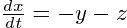
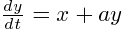
With a, b, and c set to 0.2, 0.2, and 5.7, respectively.

A short time series from the Rosseler Attractor

Poincare sections are important for visualizing an attractor that is embedded in greater than 3 spatial dimensions. Additionally, certain dynamical and topological properties are invariant to these transformations such as Lyapunov exponents and bifurcation diagrams (See Sprott 2003). However, the Lyapunov exponent with a value of 0 is lost due to the removal of the direction of the flow.

To build a Poincaré section, imagine that you have selected a slice of phase space. Every time the orbit passes through that slice, we collect a point. We repeat this over and over to create an image of what the attractor looks like in that slice of space.

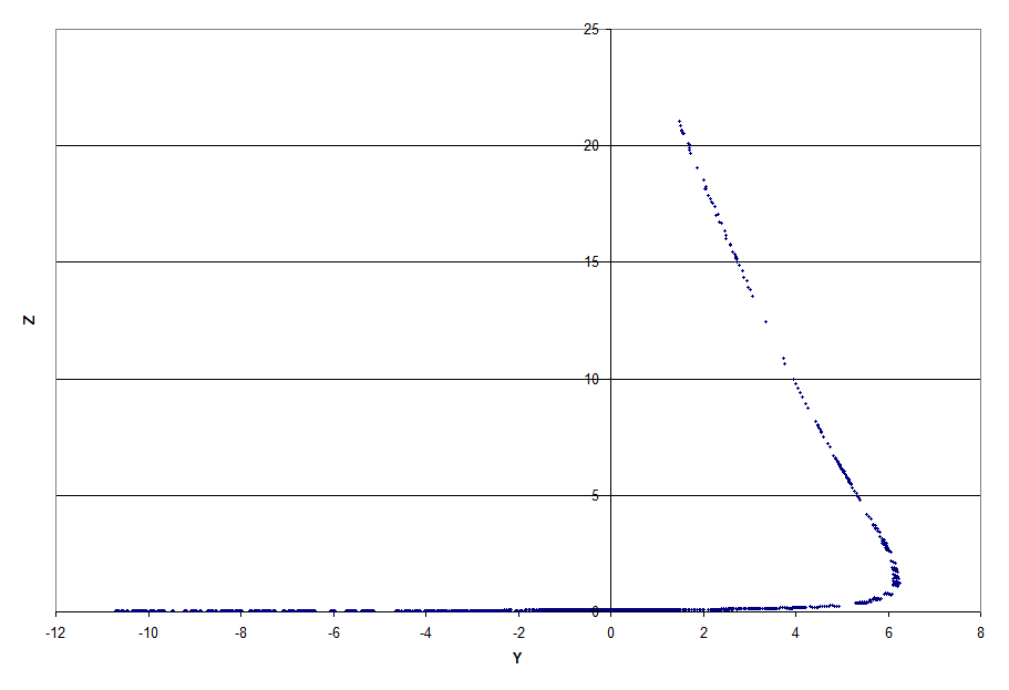
Return map for the Y and Z variables where the value of X is between 3.5 and 3.75

We can also find local maximums to create a return map. In the following graph, we look for points that are local maximums and plot them versus the previous local maximum.

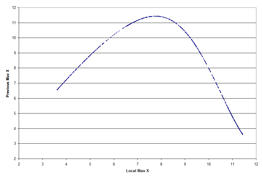
The local maxima of the variable X versus previous local maxima of the variable X

The following Python code uses the 4-th order Runge-Kutta method to create this return map.

import math, operator, random

dataX0 = []
dataY0 = []
dataZ0 = []
yList = []
xList = []
zList = []

count = 1
t = 1

x = -9
y = 0
z = 0

xList.append(x)
yList.append(y)
zList.append(z)

h = .01

a = .2
b = .2
c = 5.7

def f(x,y,z):
	global a,b,c
	dxdt = -y-z
	return dxdt

def g(x,y,z):
	global a,b,c
	dydt = x + a * y
	return dydt

def e(x,y,z):
	global a,b,c
	dzdt = b + z * (x - c)
	return dzdt

def rk4o(x, y, z):
	global h
	k1x = h*f(x, y, z)
	k1y = h*g(x, y, z)
	k1z = h*e(x, y, z)

	k2x = h*f(x + k1x/2.0, y + k1y/2.0, z + k1z/2.0)
	k2y = h*g(x + k1x/2.0, y + k1y/2.0, z + k1z/2.0)
	k2z = h*e(x + k1x/2.0, y + k1y/2.0, z + k1z/2.0)

	k3x = h*f(x + k2x/2.0, y + k2y/2.0, z + k2z/2.0)
	k3y = h*g(x + k2x/2.0, y + k2y/2.0, z + k2z/2.0)
	k3z = h*e(x + k2x/2.0, y + k2y/2.0, z + k2z/2.0)

	k4x = h*f(x + k3x, y + k3y, z + k3z)
	k4y = h*g(x + k3x, y + k3y, z + k3z)
	k4z = h*e(x + k3x, y + k3y, z + k3z)

	x = x + k1x/6.0 + k2x/3.0 + k3x/3.0 + k4x/6.0
	y = y + k1y/6.0 + k2y/3.0 + k3y/3.0 + k4y/6.0
	z = z + k1z/6.0 + k2z/3.0 + k3z/3.0 + k4z/6.0

	return [x,y,z]

X0 = []
Y0 = []
Z0 = []
previousLocalMax = x
localMax = x
t = 1
changeInTime = h
avgChange = []
LastPoint = changeInTime

while changeInTime < 20000 and len(dataX0) < 1000:
	[x,y,z] = rk4o(xList[t-1], yList[t-1], zList[t-1])

	xList.append(x)
	yList.append(y)
	zList.append(z)
	if 201 < changeInTime:

		# Print y and z points when x is between 3.5 and 3.75 (as shown in the figure)
		if x < 3.75 and x > 3.5:
			print y , "," , z

		if x < xList[t-1] and xList[t-2] < xList[t-1]:
			previousLocalMax = localMax
			localMax = xList[t-1]
			dataX0.append(localMax)
			dataY0.append(previousLocalMax)
			# Calculate the change between this and last point
			avgChange.append(changeInTime - LastPoint)
			LastPoint = changeInTime

	t = t + 1
	changeInTime += h

# Print the average steps between points
print "Average Number of Steps between points:", sum(avgChange[1:]) / float(len(avgChange[1:]))
print "First Return Map Length: "  + str(len(dataX0))
f = open("rosseler.csv", "w")
i = 0
while i < len(X0) and i < 10000:
	f.write(str(X0[i]) + "," + str(Y0[i])+ "," + str(Z0[i])+"\n")
	i = i + 1
f.close()

f = open("fr-rossler-x", "w")
i = 0
while i < len(dataX0):
	f.write(str(dataX0[i])+"\r")
	i = i + 1
f.close()